MA Crossover Strategy with TP/SL (5 EMA Filter)How the Strategy Works on a 5-Minute Chart:
Data Input (5-Minute Candles):
Every single data point (candle) on your chart will represent 5 minutes of price action (Open, High, Low, Close for that 5-minute period).
All calculations (MAs, EMA, signals) will be based on these 5-minute price data points.
Moving Average Calculations:
Fast MA (10-period SMA): This will be the Simple Moving Average of the closing prices of the last 10 five-minute candles. It reacts relatively quickly to recent price changes.
Slow MA (30-period SMA): This will be the Simple Moving Average of the closing prices of the last 30 five-minute candles. It represents a slightly longer-term trend compared to the Fast MA.
5 EMA (5-period EMA): This is the Exponential Moving Average of the closing prices of the last 5 five-minute candles. Being an EMA, it gives more weight to the most recent 5-minute prices, making it very responsive to immediate price action.
Signal Generation (Entry Conditions):
Long Entry Signal:
The 10-period SMA crosses above the 30-period SMA (indicating a potential bullish shift in the short-to-medium term trend).
AND the current 5-minute candle's closing price is above the 5-period EMA (confirming that the immediate price momentum is also bullish and supporting the crossover).
If both conditions are met at the close of a 5-minute candle, a "Buy" signal is generated.
Short Entry Signal:
The 10-period SMA crosses below the 30-period SMA (indicating a potential bearish shift).
AND the current 5-minute candle's closing price is below the 5-period EMA (confirming immediate bearish momentum).
If both conditions are met at the close of a 5-minute candle, a "Sell" signal is generated.
Trade Execution:
When a signal is triggered, the strategy enters a trade (long or short) at the closing price of that 5-minute candle.
Immediately upon entry, it places two contingent orders:
Take Profit (Target): Set at 2% (by default) away from your entry price. For a long trade, it's 2% above; for a short trade, 2% below.
Stop Loss: Set at 1% (by default) away from your entry price. For a long trade, it's 1% below; for a short trade, 1% above.
The trade will remain open until either the Take Profit or Stop Loss price is hit by subsequent 5-minute candles.
Implications for Trading on a 5-Minute Chart:
Increased Trade Frequency: You will likely see many more signals and trades compared to higher timeframes (like 1-hour or daily charts). This means more potential opportunities but also more transaction costs (commissions, slippage).
Sensitivity to Noise: Lower timeframes are more prone to "market noise" – small, random price fluctuations that don't indicate a true trend. While the 5 EMA filter helps, some false signals might still occur.
Faster Price Action: Price movements can be very rapid on a 5-minute chart. Your take profit or stop loss levels might be hit very quickly, sometimes within the same or next few candles.
Parameter Optimization is Crucial: The default MA lengths (10, 30) and EMA (5) might not be optimal for every asset or market condition on a 5-minute chart. You'll need to backtest extensively and potentially adjust these lengths, as well as the targetPerc and stopPerc, to find what works best for the specific instrument you're trading.
Risk Management: The fixed percentage stop loss is vital on a 5-minute chart due to its volatility. Without it, a few unfavorable moves could lead to significant losses.
스크립트에서 "stop loss"에 대해 찾기

TradePlanner ProPlan smarter. Trade with precision.
TradePlanner Pro is a professional-grade overlay tool designed to streamline your trading decisions by visually organizing your trade plans directly on the chart. Built for traders who value preparation and clarity, this script enables precise entry planning, risk management, and target visualization—all tailored per symbol.
Core Purpose
TradePlanner Pro helps you map out potential trades using pre-defined symbol-based presets. It dynamically calculates position sizes based on your account size or fixed risk, then visualizes key trade levels (Entry, Take Profits, Stop Loss) with profit/loss metrics in both dollar and percentage terms. It's the perfect companion for traders who prepare their setups in advance and want their plans clearly represented on the chart.
Key Features
🔹 Per-Symbol Presets: Define entries, up to 3 take-profit levels, and stop-losses for each ticker.
🔹 Dynamic Risk Sizing: Choose between percentage-based risk or fixed dollar risk per trade.
🔹 Visual Trade Mapping: Automatically plots Entry, TP1–TP3, and SL lines on your chart.
🔹 Real-Time P&L Labels: Displays profit/loss amounts and percentages, with optional R/R ratios.
🔹 Custom Investment Display: Shows how much capital is allocated per trade.
🔹 Clean, Configurable UI: Adjust label positions, font sizes, opacity, and label visibility to match your style.
Whether you're swing trading or day trading, TradePlanner Pro helps you stay disciplined, organized, and confident in your execution.
How to Use TradePlanner Pro – Step-by-Step Guide
TradePlanner Pro is designed to be easy to set up while giving you full control over how your trades are visualized and calculated. Here’s how to get started:
1. Start with Default Settings
By default, the script assumes:
Account Size: $10,000
Max Money per Trade (%): 1.0%
Max Risk (USD): 0 (disabled; only percentage risk is used)
This means the script will size each trade to risk 1% of your account balance per trade unless you override it with a fixed USD risk amount.
2. Set Up Your Symbol Presets
The "Symbol Presets" input is a flexible text area where you define trade setups for each ticker.
Format (one per line):
SYMBOL:Entry,TP1 ,SL
Example:
AAPL:250,260,270,240
MSFT:100,110,90
TSLA:180,200,170
You can include 1 to 3 take-profit levels.
The script will only activate for the current chart’s symbol, matching what's listed.
3. Customize Risk Parameters
You can use:
Account % Risk – Based on account size and % risk.
Fixed USD Risk – When a dollar amount is entered (>0), it takes priority and calculates share size based on the risk per share.
There's also an option to round share quantities down to whole units, which is useful for stock or crypto trading platforms that only allow whole-number units.
4. Choose What to Display
Toggle on/off these elements as needed:
Show Entry/TP/SL Lines
Show P&L Labels – Profit/loss amounts at each target and SL.
Show Amount Invested – Includes total dollar value in the quantity label.
Show Percentages – Adds % gain/loss to each label.
Show Risk/Reward Ratios – Optionally displayed beside or below TP labels.
You can further adjust:
Font size and label opacity
Label position offset – In percent of price range, so they don’t overlap the actual levels.
5. Read the Visual Outputs
Once the preset matches the current chart symbol:
Lines will appear for Entry, TP1-TP3, and Stop Loss.
Labels will display your:
Trade quantity (and invested amount)
Dollar and % profit at each target
Total loss at stop loss
Optional R/R ratios
Everything updates dynamically and adjusts to your current chart scale and bar availabilit

ICT Swiftedge# ICT SwiftEdge: Advanced Market Structure Trading System
**Overview**
ICT SwiftEdge is a powerful trading system built upon the foundation of ICTProTools' ICT Breakers, licensed under the Mozilla Public License 2.0 (mozilla.org). This script has been significantly enhanced by to combine market structure analysis with modern technical indicators and a sleek, AI-inspired statistics dashboard. The goal is to provide traders with a comprehensive tool for identifying high-probability trade setups, managing exits, and tracking performance in a visually intuitive way.
**Credits**
This script is a derivative work based on the original "ICT Breakers" by ICTProTools, used with permission under the Mozilla Public License 2.0. Significant enhancements, including RSI-MA signals, trend filtering, dynamic timeframe adjustments, dual exit strategies, and an AI-style statistics dashboard, were developed by . We express our gratitude to ICTProTools for their foundational work in market structure analysis.
**What It Does**
ICT SwiftEdge integrates multiple trading concepts to help traders identify and manage trades based on market structure and momentum:
- **Market Structure Analysis**: Identifies Break of Structure (BOS) and Market Structure Shift (MSS) patterns, which signal potential trend continuations or reversals. BOS indicates a continuation of the current trend, while MSS highlights a shift in market direction, providing key entry points.
- **RSI-MA Signals**: Generates "BUY" and "SELL" signals when BOS or MSS patterns align with the Relative Strength Index (RSI) smoothed by a Moving Average (RSI-MA). Signals are filtered to occur only when RSI-MA is above 50 (for buys) or below 50 (for sells), ensuring momentum supports the trade direction.
- **Trend Filtering**: Prevents multiple signals in the same trend, ensuring only one buy or sell signal per trend direction, reducing noise and improving trade clarity.
- **Dynamic Timeframe Adjustment**: Automatically adjusts pivot points, RSI, and MA parameters based on the selected chart timeframe (1M to 1D), optimizing performance across different market conditions.
- **Flexible Exit Strategies**: Offers two user-selectable exit methods:
- **Trailing Stop-Loss (TSL)**: Exits trades when price moves against the position by a user-defined distance (in points), locking in profits or limiting losses.
- **RSI-MA Exit**: Exits trades when RSI-MA crosses the 50 level, signaling a potential loss of momentum.
- Users can enable either or both strategies, providing flexibility to adapt to different trading styles.
- **AI-Style Statistics Dashboard**: Displays real-time trade performance metrics in a futuristic, neon-colored interface, including total trades, wins, losses, win/loss ratio, and win percentage. This helps traders evaluate the system's effectiveness without external tools.
**Why This Combination?**
The integration of these components creates a synergistic trading system:
- **BOS/MSS and RSI-MA**: Combining market structure breaks with RSI-MA ensures entries are based on both price action (structure) and momentum (RSI-MA), increasing the likelihood of high-probability trades.
- **Trend Filtering**: By limiting signals to one per trend, the system avoids overtrading and focuses on significant market moves.
- **Dynamic Adjustments**: Timeframe-specific parameters make the system versatile, suitable for scalping (1M, 5M) or swing trading (4H, 1D).
- **Dual Exit Strategies**: TSL protects profits during trending markets, while RSI-MA exits are ideal for range-bound or reversing markets, catering to diverse market conditions.
- **Statistics Dashboard**: Provides immediate feedback on trade performance, enabling data-driven decision-making without manual tracking.
This combination balances technical precision with user-friendly visuals, making it accessible to both novice and experienced traders.
**How to Use**
1. **Add to Chart**: Apply the script to any TradingView chart.
2. **Configure Settings**:
- **Chart Timeframe**: Select your chart's timeframe (1M to 1D) to optimize parameters.
- **Structure Timeframe**: Choose a timeframe for market structure analysis (leave blank for chart timeframe).
- **Exit Strategy**: Enable Trailing Stop-Loss (`useTslExit`), RSI-MA Exit (`useRsiMaExit`), or both. Adjust `tslPoints` for TSL distance.
- **Show Signals/Labels**: Toggle `showSignals` and `showExit` to display "BUY", "SELL", and "EXIT" labels.
- **Dashboard**: Enable `showDashboard` to view trade statistics. Customize colors with `dashboardBgColor` and `dashboardTextColor`.
3. **Trading**:
- Look for "BUY" or "SELL" labels to enter trades when BOS/MSS aligns with RSI-MA.
- Exit trades at "EXIT" labels based on your chosen strategy.
- Monitor the statistics dashboard to track performance (total trades, win/loss ratio, win percentage).
4. **Alerts**: Set up alerts for BOS, MSS, buy, sell, or exit signals using the provided alert conditions.
**License**
This script is licensed under the Mozilla Public License 2.0 (mozilla.org). The source code is available for review and modification under the terms of this license.
**Compliance with TradingView House Rules**
This publication adheres to TradingView's House Rules and Scripts Publication Rules. It provides a clear, self-contained description of the script's functionality, credits the original author (ICTProTools), and explains the rationale for combining indicators. The script contains no promotional content, offensive language, or proprietary restrictions beyond MPL 2.0.
**Note**
Trading involves risk, and past performance is not indicative of future results. Always backtest and validate the system on your preferred markets and timeframes before live trading.
Enjoy trading with ICT SwiftEdge, and let data-driven insights guide your decisions!

Trend Zone Moving Averages📈 Trend Zone Moving Averages
The Trend Zone Moving Averages indicator helps traders quickly identify market trends using the 50SMA, 100SMA, and 200SMA. With dynamic background colors, customizable settings, and real-time alerts, this tool provides a clear view of bullish, bearish, and extreme trend conditions.
🔹 Features:
Trend Zones with Dynamic Background Colors
Green → Bullish Trend (50SMA > 100SMA > 200SMA, price above 50SMA)
Red → Bearish Trend (50SMA < 100SMA < 200SMA, price below 50SMA)
Yellow → Neutral Trend (Mixed signals)
Dark Green → Extreme Bullish (Price above all three SMAs)
Dark Red → Extreme Bearish (Price below all three SMAs)
Customizable Moving Averages
Toggle 50SMA, 100SMA, and 200SMA on/off from the settings.
Perfect for traders who prefer a cleaner chart.
Real-Time Trend Alerts
Get instant notifications when the trend changes:
🟢 Bullish Zone Alert – When price enters a bullish trend.
🔴 Bearish Zone Alert – When price enters a bearish trend.
🟡 Neutral Zone Alert – When trend shifts to neutral.
🌟 Extreme Bullish Alert – When price moves above all SMAs.
⚠️ Extreme Bearish Alert – When price drops below all SMAs.
✅ Perfect for Any Market
Works on stocks, forex, crypto, and commodities.
Adaptable for day traders, swing traders, and investors.
⚙️ How to Use: Trend Zone Moving Averages Strategy
This strategy helps traders identify and trade with the trend using the Trend Zone Moving Averages indicator. It works across stocks, forex, crypto, and commodities.
🟢 Bullish Trend Strategy (Green Background)
Objective: Look for buying opportunities when the market is in an uptrend.
Entry Conditions:
✅ Background is Green (Bullish Zone).
✅ Price is above the 50SMA (confirming strength).
✅ Price pulls back to the 50SMA and bounces OR breaks above a key resistance level.
Stop Loss:
🔹 Place below the most recent swing low or just under the 50SMA.
Take Profit:
🔹 First target at the next resistance level or recent swing high.
🔹 Second target if price continues higher—trail stops to lock in profits.
🔴 Bearish Trend Strategy (Red Background)
Objective: Look for shorting opportunities when the market is in a downtrend.
Entry Conditions:
✅ Background is Red (Bearish Zone).
✅ Price is below the 50SMA (confirming weakness).
✅ Price pulls back to the 50SMA and rejects OR breaks below a key support level.
Stop Loss:
🔹 Place above the most recent swing high or just above the 50SMA.
Take Profit:
🔹 First target at the next support level or recent swing low.
🔹 Second target if price keeps falling—trail stops to secure profits.
🌟 Extreme Trend Strategy (Dark Green / Dark Red Background)
Objective: Trade with momentum when the market is in a strong trend.
Entry Conditions:
✅ Dark Green Background → Extreme Bullish: Price is above all three SMAs (strong uptrend).
✅ Dark Red Background → Extreme Bearish: Price is below all three SMAs (strong downtrend).
Trade Execution:
🔹 For longs (Dark Green): Look for breakout entries above resistance or pullbacks to the 50SMA.
🔹 For shorts (Dark Red): Look for breakdown entries below support or rejections at the 50SMA.
Risk Management:
🔹 Use tighter stop losses and trail profits aggressively to maximize gains.
🟡 Neutral Trend Strategy (Yellow Background)
Objective: Avoid trading or wait for a breakout.
What to Do:
🔹 Avoid trading in this zone—price is indecisive.
🔹 Wait for confirmation (background turns green/red) before taking a trade.
🔹 Use alerts to notify you when the trend resumes.
📌 Final Tips
Use this strategy with price action for extra confirmation.
Combine with support/resistance levels to improve accuracy.
Set alerts for trend changes so you never miss an opportunity.
Enjoy!

Simple APF Strategy Backtesting [The Quant Science]Simple backtesting strategy for the quantitative indicator Autocorrelation Price Forecasting. This is a Buy & Sell strategy that operates exclusively with long orders. It opens long positions and generates profit based on the future price forecast provided by the indicator. It's particularly suitable for trend-following trading strategies or directional markets with an established trend.
Main functions
1. Cycle Detection: Utilize autocorrelation to identify repetitive market behaviors and cycles.
2. Forecasting for Backtesting: Simulate trades and assess the profitability of various strategies based on future price predictions.
Logic
The strategy works as follow:
Entry Condition: Go long if the hypothetical gain exceeds the threshold gain (configurable by user interface).
Position Management: Sets a take-profit level based on the future price.
Position Sizing: Automatically calculates the order size as a percentage of the equity.
No Stop-Loss: this strategy doesn't includes any stop loss.
Example Use Case
A trader analyzes a dayli period using 7 historical bars for autocorrelation.
Sets a threshold gain of 20 points using a 5% of the equity for each trade.
Evaluates the effectiveness of a long-only strategy in this period to assess its profitability and risk-adjusted performance.
User Interface
Length: Set the length of the data used in the autocorrelation price forecasting model.
Thresold Gain: Minimum value to be considered for opening trades based on future price forecast.
Order Size: percentage size of the equity used for each single trade.
Strategy Limit
This strategy does not use a stop loss. If the price continues to drop and the future price forecast is incorrect, the trader may incur a loss or have their capital locked in the losing trade.
Disclaimer!
This is a simple template. Use the code as a starting point rather than a finished solution. The script does not include important parameters, so use it solely for educational purposes or as a boilerplate.

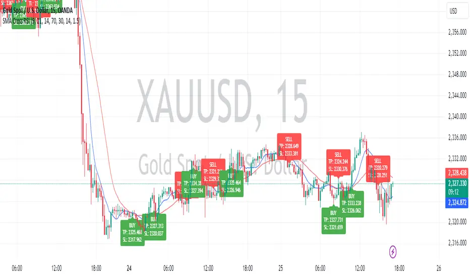
SMA Crossover with RSI ConfirmationThis is a sniper entry indicator that provides Buy and Sell signals using other Indicators to give the best possible Entries
Moving Average Crossovers:
The indicator uses two moving averages: a short-term SMA (Simple Moving Average) and a long-term SMA.
When the short-term SMA crosses above the long-term SMA, it generates a buy signal (indicating potential upward momentum).
When the short-term SMA crosses below the long-term SMA, it generates a sell signal (indicating potential downward momentum).
RSI Confirmation:
The indicator incorporates RSI (Relative Strength Index) to confirm the buy and sell signals generated by the moving average crossovers.
RSI is used to gauge the overbought and oversold conditions of the market.
A buy signal is confirmed if RSI is below a specified overbought level, indicating potential buying opportunity.
A sell signal is confirmed if RSI is above a specified oversold level, indicating potential selling opportunity.
Dynamic Take Profit and Stop Loss:
The indicator calculates dynamic take profit and stop loss levels based on the Average True Range (ATR).
ATR is used to gauge market volatility, and the take profit and stop loss levels are adjusted accordingly.
This feature helps traders to manage their risk effectively by setting appropriate profit targets and stop loss levels.
Combining the information provided by these, the indicator will provide an entry point with a provided take profit and stop loss. The indicator can be applied to different asset classes. Risk management must be applied when using this indicator as it is not 100% guaranteed to be profitable.

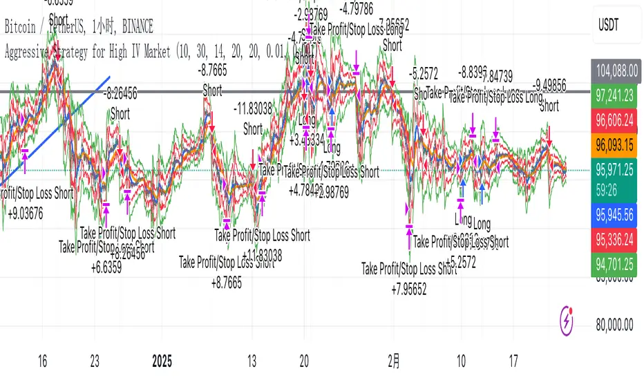
Aggressive Strategy for High IV Market### Strategic background
In a volatile high IV market, prices are volatile and market expectations of future uncertainty are high. This environment provides opportunities for aggressive trading strategies, but also comes with a high level of risk. In pursuit of a high Sharpe ratio (i.e., risk-adjusted return), we need to design a strategy that captures the benefits of market volatility while effectively controlling risk. Based on daily line cycles, I choose a combination of trend tracking and volatility filtering for highly volatile assets such as stocks, futures or cryptocurrencies.
---
### Strategy framework
#### Data
- Use daily data, including opening, closing, high and low prices.
- Suitable for highly volatile markets such as technology stocks, cryptocurrencies or volatile index futures.
#### Core indicators
1. ** Trend Indicators ** :
Fast Exponential Moving Average (EMA_fast) : 10-day EMA, used to capture short-term trends.
- Slow Exponential Moving Average (EMA_slow) : 30-day EMA, used to determine the long-term trend.
2. ** Volatility Indicators ** :
Average true Volatility (ATR) : 14-day ATR, used to measure market volatility.
- ATR mean (ATR_mean) : A simple moving average of the 20-day ATR that serves as a volatility benchmark.
- ATR standard deviation (ATR_std) : The standard deviation of the 20-day ATR, which is used to judge extreme changes in volatility.
#### Trading logic
The strategy is based on a trend following approach of double moving averages and filters volatility through ATR indicators, ensuring that trading only in a high-volatility environment is in line with aggressive and high sharpe ratio goals.
---
### Entry and exit conditions
#### Admission conditions
- ** Multiple entry ** :
- EMA_fast Crosses EMA_slow (gold cross), indicating that the short-term trend is turning upward.
-ATR > ATR_mean + 1 * ATR_std indicates that the current volatility is above average and the market is in a state of high volatility.
- ** Short Entry ** :
- EMA_fast Crosses EMA_slow (dead cross) downward, indicating that the short-term trend turns downward.
-ATR > ATR_mean + 1 * ATR_std, confirming high volatility.
#### Appearance conditions
- ** Long show ** :
- EMA_fast Enters the EMA_slow (dead cross) downward, and the trend reverses.
- or ATR < ATR_mean-1 * ATR_std, volatility decreases significantly and the market calms down.
- ** Bear out ** :
- EMA_fast Crosses the EMA_slow (gold cross) on the top, and the trend reverses.
- or ATR < ATR_mean-1 * ATR_std, the volatility is reduced.
---
### Risk management
To control the high risk associated with aggressive strategies, set up the following mechanisms:
1. ** Stop loss ** :
- Long: Entry price - 2 * ATR.
- Short: Entry price + 2 * ATR.
- Dynamic stop loss based on ATR can adapt to market volatility changes.
2. ** Stop profit ** :
- Fixed profit target can be selected (e.g. entry price ± 4 * ATR).
- Or use trailing stop losses to lock in profits following price movements.
3. ** Location Management ** :
- Reduce positions appropriately in times of high volatility, such as dynamically adjusting position size according to ATR, ensuring that the risk of a single trade does not exceed 1%-2% of the account capital.
---
### Strategy features
- ** Aggressiveness ** : By trading only in a high ATR environment, the strategy takes full advantage of market volatility and pursues greater returns.
- ** High Sharpe ratio potential ** : Trend tracking combined with volatility filtering to avoid ineffective trades during periods of low volatility and improve the ratio of return to risk.
- ** Daily line Cycle ** : Based on daily line data, suitable for traders who operate frequently but are not too complex.
---
### Implementation steps
1. ** Data Preparation ** :
- Get the daily data of the target asset.
- Calculate EMA_fast (10 days), EMA_slow (30 days), ATR (14 days), ATR_mean (20 days), and ATR_std (20 days).
2. ** Signal generation ** :
- Check EMA cross signals and ATR conditions daily to generate long/short signals.
3. ** Execute trades ** :
- Enter according to the signal, set stop loss and profit.
- Monitor exit conditions and close positions in time.
4. ** Backtest and Optimization ** :
- Use historical data to backtest strategies to evaluate Sharpe ratios, maximum retracements, and win rates.
- Optimize parameters such as EMA period and ATR threshold to improve policy performance.
---
### Precautions
- ** Trading costs ** : Highly volatile markets may result in frequent trading, and the impact of fees and slippage on earnings needs to be considered.
- ** Risk Control ** : Aggressive strategies may face large retracements and need to strictly implement stop losses.
- ** Scalability ** : Additional metrics (such as volume or VIX) can be added to enhance strategy robustness, or combined with machine learning to predict trends and volatility.
---
### Summary
This is a trend following strategy based on dual moving averages and ATR, designed for volatile high IV markets. By entering into high volatility and exiting into low volatility, the strategy combines aggressive and risk-adjusted returns for traders seeking a high sharpe ratio. It is recommended to fully backtest before implementation and adjust the parameters according to the specific market.
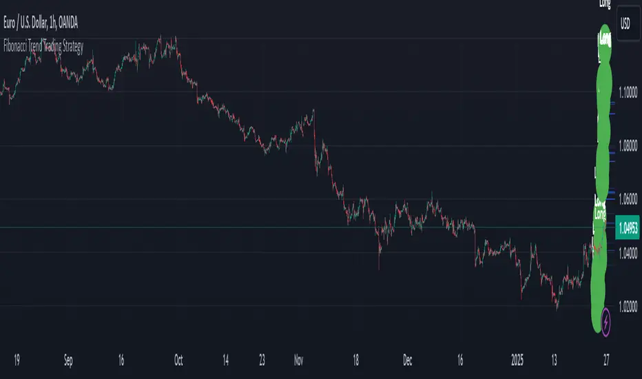
Fibonacci Extension Strt StrategyCore Logic and Steps:
Weekly Trend Identification:
Find the last significant Higher High (HH) and Lower Low (LL) or vice-versa on the Weekly timeframe.
Determine if it's an uptrend (HH followed by LL) or a downtrend (LL followed by HH).
Plot a Fibonacci Extension (or Retracement in reverse order) from the swing point determined to the other significant swing point.
Weekly Retracement Levels:
Display horizontal lines at the 0.236, 0.382, and 0.5 Fibonacci levels from the weekly extension.
Monitor price action on these levels.
Daily Confirmation:
When price hits the Fib levels, examine the Daily chart.
Look for a rejection wick (indicating the pull back is ending) on the identified weekly retracement levels.
Confirm that the price is indeed starting to continue in the direction of the original weekly trend.
Four-Hour Entry:
On the 4H timeframe, plot a new Fib Extension in the opposite direction of the weekly.
If it's an uptrend, the Fib is plotted from last swing low to its swing high. If the weekly trend was bearish the Fib will be plotted from last swing high to the swing low.
Generate an entry when price breaks the high of that candle.
Trade Management:
Entry is on the breakout of the current candle.
Stop Loss: Place the stop loss below the wick of the breakout candle.
Take Profit 1: Close 50% of the position at the 0.5 Fibonacci level. Move the stop loss to breakeven on this position.
Take Profit 2: Close another 25% of the position at the 0.236 Fib level.
Trailing Take Profit: Keep the last 25% open, using a trailing stop loss. (You'll need to define the logic for the trailing stop, e.g., trailing stop using the last high/low)
How to Use in TradingView:
Open a TradingView Chart.
Click on "Pine Editor" at the bottom.
Copy and paste the corrected Pine Script code.
Click "Add to Chart".
The indicator should now be displayed on your chart.
Long Position with 1:3 Risk Reward and 20EMA CrossoverThe provided Pine Script code implements a strategy to identify long entry signals based on a 20-EMA crossover on a 5-minute timeframe. Once a buy signal is triggered, it calculates and plots the following:
Entry Price: The price at which the buy signal is generated.
Stop Loss: The low of the previous candle, acting as a risk management tool.
Take Profit: The price level calculated based on a 1:3 risk-reward ratio.
Key Points:
Buy Signal: A buy signal is generated when the current 5-minute candle closes above the 20-EMA.
Risk Management: The stop-loss is set below the entry candle to limit potential losses.
Profit Target: The take-profit is calculated based on a 1:3 risk-reward ratio, aiming for a potential profit three times the size of the risk.
Visualization: The script plots the entry price, stop-loss, and take-profit levels on the chart for visual clarity.
Remember:
Backtesting: It's crucial to backtest this strategy on historical data to evaluate its performance and optimize parameters.
Risk Management: Always use appropriate risk management techniques, such as stop-loss orders and position sizing, to protect your capital.
Market Conditions: Market conditions can change, and strategies that worked in the past may not perform as well in the future. Continuously monitor and adapt your strategy.
By understanding the core components of this script and applying sound risk management principles, you can effectively use it to identify potential long entry opportunities in the market.

Ask-Weighted Averages This indicator provides two price-based reference lines derived from volume dynamics within each bar. Specifically, it calculates a volume-weighted average price using only the portion of trading volume that occurred on the "ask" side, implying more aggressive buying activity. The logic behind this approach is to highlight potential support and resistance levels where buyers have shown greater conviction.
Key Features:
Ask-Weighted Average Prices:
Instead of using the entire trade volume, the lines focus on "ask volume" (volume associated with trades occurring at or near the ask price). This helps to spotlight areas where buyers have been dominant, potentially revealing more meaningful price levels for future market behavior.
Conditional vs. Continuous Lines:
Conditional Line: This line is only plotted if the dollar volume (a rough measure of trade value) exceeds a specified threshold, ensuring that the highlighted level is backed by substantial trading activity.
Continuous Line: A second line is always displayed, providing a running ask-weighted average price reference for additional context, regardless of dollar volume.
Supports Identifying Key Price Zones:
By focusing on where more motivated buyers have been active, the indicator helps traders identify potential inflection points in price, such as areas where the market might find support on pullbacks or resistance during rallies.
Overall, this indicator serves as a specialized tool for traders interested in volume-driven price analysis. It aims to refine the understanding of where buyers are most engaged and how that might shape future price movements.
Risks Associated with Trading:
No indicator can guarantee profitable trades or accurately predict future price movements. Market conditions are inherently unpredictable, and reliance on any single tool or combination of tools carries the risk of financial loss. Traders should practice sound risk management, including the use of stop losses and position sizing, and should not trade with funds they cannot afford to lose. Ultimately, decisions should be guided by a thorough trading plan and possibly supplemented with other forms of market analysis or professional advice.
Risks and Important Considerations:
• Not a Standalone Tool:
• This indicator should not be used in isolation. It is essential to incorporate additional technical analysis tools, fundamental analysis, and market context when making trading decisions.
• Relying solely on this indicator may lead to incomplete assessments of market conditions.
• Market Volatility and False Signals:
• Financial markets can be highly volatile, and indicators based on historical data may not accurately predict future movements.
• The indicator may produce false signals due to sudden market changes, low liquidity, or atypical trading activity.
• Risk Management:
• Always employ robust risk management strategies, including setting stop-loss orders, diversifying your portfolio, and not over-leveraging positions.
• Understand that no indicator guarantees success, and losses are a natural part of trading.
• Emotional Discipline:
• Avoid making impulsive decisions based on indicator signals alone.
• Emotional trading can lead to significant financial losses; maintain discipline and adhere to a well-thought-out trading plan.
• Continuous Learning and Adaptation:
• Stay informed about market news, economic indicators, and global events that may impact trading conditions.
• Continuously evaluate and adjust your trading strategies as market dynamics evolve.
• Consultation with Professionals:
• Consider seeking advice from financial advisors or professional traders to understand better how this indicator can fit into your overall trading strategy.
• Professional guidance can provide personalized insights based on your financial goals and risk tolerance.
Disclaimer:
Trading financial instruments involves substantial risk and may not be suitable for all investors. Past performance is not indicative of future results. This indicator is provided for informational and educational purposes only and should not be considered investment advice. Always conduct your own research and consult with a licensed financial professional before making any trading decisions.
Note: The effectiveness of any technical indicator can vary based on market conditions and individual trading styles. It's crucial to test indicators thoroughly using historical data and possibly paper trading before applying them in live trading scenarios.

WhalenatorThis custom TradingView indicator combines multiple analytic techniques to help identify potential market trends, areas of support and resistance, and zones of heightened trading activity. It incorporates a SuperTrend-like line based on ATR, Keltner Channels for volatility-based price envelopes, and dynamic order blocks derived from significant volume and pivot points. Additionally, it highlights “whale” activities—periods of exceptionally large volume—along with an estimated volume profile level and approximate bid/ask volume distribution. Together, these features aim to offer traders a more comprehensive view of price structure, volatility, and institutional participation.
This custom TradingView indicator integrates multiple trading concepts into a single, visually descriptive tool. Its primary goal is to help traders identify directional bias, volatility levels, significant volume events, and potential support/resistance zones on a price chart. Below are the main components and their functionalities:
SuperTrend-Like Line (Trend Bias):
At the core of the indicator is a trend-following line inspired by the SuperTrend concept, which uses Average True Range (ATR) to adaptively set trailing stop levels. By comparing price to these levels, the line attempts to indicate when the market is in an uptrend (price above the line) or a downtrend (price below the line). The shifting levels can provide a dynamic sense of direction and help traders stay with the predominant trend until it shifts.
Keltner Channels (Volatility and Range):
Keltner Channels, based on an exponential moving average and Average True Range, form volatility-based envelopes around price. They help traders visualize whether price is extended (touching or moving outside the upper/lower band) or trading within a stable range. This can be useful in identifying low-volatility consolidations and high-volatility breakouts.
Dynamic Order Blocks (Approximations of Supply/Demand Zones):
By detecting pivot highs and lows under conditions of significant volume, the indicator approximates "order blocks." Order blocks are areas where institutional buying or selling may have occurred, potentially acting as future support or resistance zones. Although these approximations are not perfect, they offer a visual cue to areas on the chart where price might react strongly if revisited.
Volume Profile Proxy and Whale Detection:
The indicator highlights price levels associated with recent maximum volume activity, providing a rough "volume profile" reference. Such levels often become key points of price interaction.
"Whale" detection logic attempts to identify bars where exceptionally large volume occurs (beyond a defined threshold). By tracking these "whale bars," traders can infer where heavy participation—often from large traders or institutions—may influence market direction or create zones of interest.
Approximate Bid/Ask Volume and Dollar Volume Tracking:
The script estimates whether volume within each bar leans more towards the bid or the ask side, aiming to understand which participant (buyers or sellers) might have been more aggressive. Additionally, it calculates dollar volume (close price multiplied by volume) and provides an average to gauge the relative participation strength over time.
Labeling and Visual Aids:
Dynamic labels display Whale Frequency (the ratio of bars with exceptionally large volume), average dollar volume, and approximate ask/bid volume metrics. This gives traders at-a-glance insights into current market conditions, participation, and sentiment.
Strengths:
Multifaceted Analysis:
By combining trend, volatility, volume, and order block logic in one place, the indicator saves chart space and simplifies the analytical process. Traders gain a holistic view without flipping between multiple separate tools.
Adaptable to Market Conditions:
The use of ATR and Keltner Channels adapts to changing volatility conditions. The SuperTrend-like line helps keep traders aligned with the prevailing trend, avoiding constant whipsaws in choppy markets.
Volume-Based Insights:
Integrating whale detection and a crude volume profile proxy helps traders understand where large players might be interacting. This perspective can highlight critical levels that might not be evident from price action alone.
Convenient Visual Cues and Labels:
The indicator provides quick reference points and textual information about the underlying volume dynamics, making decision-making potentially faster and more informed.
Weaknesses:
Heuristic and Approximate Nature:
Many of the indicator’s features, like the "order blocks," "whale detection," and the approximate bid/ask volume, rely on heuristics and assumptions that may not always be accurate. Without actual Level II data or true volume profiles, the insights are best considered as supplementary, not definitive signals.
Lagging Components:
Indicators that rely on past data, like ATR-based trends or moving averages for Keltner Channels, inherently lag behind price. This can cause delayed signals, particularly in fast-moving markets, potentially missing some early opportunities or late in confirming market reversals.
No Guaranteed Predictive Power:
As with any technical tool, it does not forecast the future with certainty. Strong volume at a certain level or a bullish SuperTrend reading does not guarantee price will continue in that direction. Market conditions can change unexpectedly, and false signals will occur.
Complexity and Overreliance Risk:
With multiple signals combined, there’s a risk of information overload. Traders might feel compelled to rely too heavily on this one tool. Without complementary analysis (fundamentals, news, or additional technical confirmation), overreliance on the indicator could lead to misguided trades.
Conclusion:
This integrated indicator offers a comprehensive visual guide to market structure, volatility, and activity. Its strength lies in providing a multi-dimensional viewpoint in a single tool. However, traders should remain aware of its approximations, inherent lags, and the potential for conflicting signals. Sound risk management, position sizing, and the use of complementary analysis methods remain essential for trading success.
Risks Associated with Trading:
No indicator can guarantee profitable trades or accurately predict future price movements. Market conditions are inherently unpredictable, and reliance on any single tool or combination of tools carries the risk of financial loss. Traders should practice sound risk management, including the use of stop losses and position sizing, and should not trade with funds they cannot afford to lose. Ultimately, decisions should be guided by a thorough trading plan and possibly supplemented with other forms of market analysis or professional advice.
Risks and Important Considerations:
• Not a Standalone Tool:
• This indicator should not be used in isolation. It is essential to incorporate additional technical analysis tools, fundamental analysis, and market context when making trading decisions.
• Relying solely on this indicator may lead to incomplete assessments of market conditions.
• Market Volatility and False Signals:
• Financial markets can be highly volatile, and indicators based on historical data may not accurately predict future movements.
• The indicator may produce false signals due to sudden market changes, low liquidity, or atypical trading activity.
• Risk Management:
• Always employ robust risk management strategies, including setting stop-loss orders, diversifying your portfolio, and not over-leveraging positions.
• Understand that no indicator guarantees success, and losses are a natural part of trading.
• Emotional Discipline:
• Avoid making impulsive decisions based on indicator signals alone.
• Emotional trading can lead to significant financial losses; maintain discipline and adhere to a well-thought-out trading plan.
• Continuous Learning and Adaptation:
• Stay informed about market news, economic indicators, and global events that may impact trading conditions.
• Continuously evaluate and adjust your trading strategies as market dynamics evolve.
• Consultation with Professionals:
• Consider seeking advice from financial advisors or professional traders to understand better how this indicator can fit into your overall trading strategy.
• Professional guidance can provide personalized insights based on your financial goals and risk tolerance.
Disclaimer:
Trading financial instruments involves substantial risk and may not be suitable for all investors. Past performance is not indicative of future results. This indicator is provided for informational and educational purposes only and should not be considered investment advice. Always conduct your own research and consult with a licensed financial professional before making any trading decisions.
Note: The effectiveness of any technical indicator can vary based on market conditions and individual trading styles. It's crucial to test indicators thoroughly using historical data and possibly paper trading before applying them in live trading scenarios.

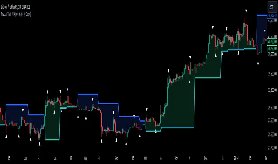
Fractal Trail [UAlgo]The Fractal Trail is designed to identify and utilize Williams fractals as dynamic trailing stops. This tool serves traders by marking key fractal points on the chart and leveraging them to create adaptive stop-loss trails, enhancing risk management and trade decision-making.
Williams fractals are pivotal in identifying potential reversals and critical support/resistance levels. By plotting fractals dynamically and providing configurable options, this indicator allows for personalized adjustments based on the trader's strategy.
This script integrates both visual fractal markers and adjustable trailing stops, offering insights into market trends while catering to a wide variety of trading styles and timeframes.
🔶 Key Features
Williams Fractals Identification: The indicator marks Williams Fractals on the chart, which are significant highs and lows within a specified range. These fractals are crucial for identifying potential reversal points in the market.
Dynamic Trailing Stops: The indicator generates dynamic trailing stops based on the identified fractals. These stops adjust automatically as new fractals are formed, providing a responsive and adaptive approach to risk management.
Fractal Range: Users can specify the number of bars to the left and right for analyzing fractals, allowing for flexibility in identifying significant price points.
Trail Buffer Percentage: A percentage-based safety margin can be added between the fractal price and the trailing stop, providing additional control over risk management.
Trail Invalidation Source: Users can choose whether the trailing stop flips based on candle closing prices or the extreme points (high/low) of the candles.
Alerts and Notifications: The indicator provides alerts for when the price crosses the trailing stops, as well as when new Williams Fractals are confirmed. These alerts can be customized to fit the trader's notification preferences.
🔶 Interpreting the Indicator
Fractal Markers: The triangles above and below the bars indicate Williams Fractals. These markers help traders identify potential reversal points in the market.
Trailing Stops: The dynamic trailing stops are plotted as lines on the chart. These lines adjust based on the latest identified fractals, providing a visual representation of potential support and resistance levels.
Fill Colors: The optional fill colors between the trailing stops and the price action help traders quickly identify the current trend and potential pullback zones.
🔶 Disclaimer
Use with Caution: This indicator is provided for educational and informational purposes only and should not be considered as financial advice. Users should exercise caution and perform their own analysis before making trading decisions based on the indicator's signals.
Not Financial Advice: The information provided by this indicator does not constitute financial advice, and the creator (UAlgo) shall not be held responsible for any trading losses incurred as a result of using this indicator.
Backtesting Recommended: Traders are encouraged to backtest the indicator thoroughly on historical data before using it in live trading to assess its performance and suitability for their trading strategies.
Risk Management: Trading involves inherent risks, and users should implement proper risk management strategies, including but not limited to stop-loss orders and position sizing, to mitigate potential losses.
No Guarantees: The accuracy and reliability of the indicator's signals cannot be guaranteed, as they are based on historical price data and past performance may not be indicative of future results.
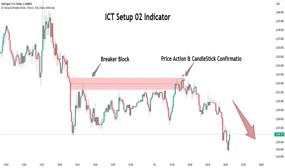
ICT Setup 02 [TradingFinder] Breaker Blocks + Reversal Candles🔵 Introduction
The "Breaker Block" concept, widely utilized in ICT (Inner Circle Trader) technical analysis, is a crucial tool for identifying reversal points and significant market shifts. Originating from the "Order Block" concept, Breaker Blocks help traders pinpoint support and resistance levels. These blocks are essential for understanding market trends and recognizing optimal entry and exit points.
A Breaker Block is essentially a failed Order Block that changes its role when price action breaks through it. When an Order Block fails to hold as a support or resistance level, it reverses its function, becoming a Breaker Block.
There are two primary types : Bullish Breaker Blocks and Bearish Breaker Blocks. These Breaker Blocks align with the prevailing market trend and indicate potential entry points after a liquidity sweep or a shift in market structure.
Understanding and applying the Breaker Block strategy enables traders to capitalize on the behavior of institutional investors, enhancing their trading outcomes.
Bullish Setup :
Bearish Setup :
🔵 How to Use
The ICT Setup 02 indicator designed to automate the identification of Bullish and Bearish Breaker Blocks. This tool enables traders to easily spot these blocks on a chart and utilize them for entering or exiting trades. Below is a breakdown of how to use this indicator in both bullish and bearish setups.
🟣 Bullish Breaker Block Setup
A Bullish Breaker Block setup is identified in an uptrend, where it serves as a potential entry point. This setup occurs when a Bearish Order Block fails and the price moves above the high of that Order Block. In this scenario, the previously bearish Order Block turns into a Bullish Breaker Block, which now acts as a support level for the price.
To trade a Bullish Breaker Block, wait for the price to retest this newly formed support level. Confirmation of the uptrend can be achieved by analyzing lower time frames for further market structure shifts or other bullish indicators.
A successful retest of the Bullish Breaker Block provides a high-probability entry point for a long trade, as it signals institutional support. Traders often place their stop-loss below the low of the Breaker Block zone to minimize risk.
🟣 Bearish Breaker Block Setup
A Bearish Breaker Block setup, conversely, is used in a downtrend to identify potential sell opportunities. This setup forms when a Bullish Order Block fails, and the price moves below the low of that Order Block.
Once this Order Block is broken, it reverses its role and becomes a Bearish Breaker Block, providing resistance to the price as it pushes downward. For a Bearish Breaker Block trade, wait for the price to retest this resistance level.
A confirmation of the downtrend, such as a market structure shift on a lower time frame or additional bearish signals, strengthens the setup. The Bearish Breaker Block retest provides an opportunity to enter a short position, with a stop-loss placed just above the high of the Breaker Block zone.
🔵 Settings
Pivot Period : This setting controls the look-back period used to identify pivot points that contribute to the detection of Order Blocks. A higher period captures longer-term pivots, while a lower period focuses on more recent price action. Adjusting this parameter allows traders to fine-tune the indicator to match their trading time frame.
Breaker Block Validity Period : This setting defines how long a Breaker Block remains valid based on the number of bars elapsed since its formation. Increasing the validity period keeps Breaker Blocks active for a longer duration, which can be useful for higher time frame analysis.
Mitigation Level BB : This option lets traders choose the level of the Order Block at which the price is expected to react. Options like "Proximal," "50% OB," and "Distal" adjust the zone where a reaction may occur, offering flexibility in setting up the entry and stop-loss levels.
Breaker Block Refinement : The refinement option refines the Breaker Block zone to display a more precise range for aggressive or defensive trading approaches. The "Aggressive" mode provides a tighter range for risk-tolerant traders, while the "Defensive" mode expands the zone for those with a more conservative approach.
🔵 Conclusion
The Breaker Block indicator provides traders with a sophisticated tool for identifying key reversal zones in the market. By leveraging Breaker Blocks, traders can gain insights into institutional order flow and predict critical support and resistance levels.
Using Breaker Blocks in conjunction with other ICT concepts, like Fair Value Gaps or liquidity sweeps, enhances the reliability of trading signals. This indicator empowers traders to make informed decisions, aligning their trades with institutional moves in the market.
As with any trading strategy, it is crucial to incorporate proper risk management, using stop-losses and position sizing to minimize potential losses. The Breaker Block strategy, when applied with discipline and thorough analysis, serves as a powerful addition to any trader’s toolkit.
PERFECT PIVOT RANGE DR ABIRAM SIVPRASAD (PPR)PERFECT PIVOT RANGE (PPR) by Dr. Abhiram Sivprasad
The Perfect Pivot Range (PPR) indicator is designed to provide traders with a comprehensive view of key support and resistance levels based on pivot points across different timeframes. This versatile tool allows users to visualize daily, weekly, and monthly pivots along with high and low levels from previous periods, helping traders identify potential areas of price reversals or breakouts.
Features:
Multi-Timeframe Pivots:
Daily, weekly, and monthly pivot levels (Pivot Point, Support 1 & 2, Resistance 1 & 2).
Helps traders understand price levels across various timeframes, from short-term (daily) to long-term (monthly).
Previous High-Low Levels:
Displays the previous week, month, and day high-low levels to highlight key zones of historical support and resistance.
Traders can easily see areas of price action from prior periods, giving context for future price movements.
Customizable Options:
Users can choose which pivot levels and high-lows to display, allowing for flexibility based on trading preferences.
Visual settings can be toggled on and off to suit different trading strategies and timeframes.
Real-Time Data:
All pivot points and levels are dynamically calculated based on real-time price data, ensuring accurate and up-to-date information for decision-making.
How to Use:
Pivot Points: Use daily, weekly, or monthly pivot points to find potential support or resistance levels. Prices above the pivot suggest bullish sentiment, while prices below indicate bearishness.
Previous High-Low: The high-low levels from previous days, weeks, or months can serve as critical zones where price may reverse or break through, indicating potential trade entries or exits.
Confluence: When pivot points or high-low levels overlap across multiple timeframes, they become even stronger levels of support or resistance.
This indicator is suitable for all types of traders (scalpers, swing traders, and long-term investors) looking to enhance their technical analysis and make more informed trading decisions.
Here are three detailed trading strategies for using the Perfect Pivot Range (PPR) indicator for options, stocks, and commodities:
1. Options Buying Strategy with PPR Indicator
Strategy: Buying Call and Put Options Based on Pivot Breakouts
Objective: To capitalize on sharp price movements when key pivot levels are breached, leading to high returns with limited risk in options trading.
Timeframe: 15-minute to 1-hour chart for intraday option trading.
Steps:
Identify the Key Levels:
Use weekly pivots for intraday trading, as they provide more significant levels for options.
Enable the "Previous Week High-Low" to gauge support and resistance from the previous week.
Call Option Setup (Bullish Breakout):
Condition: If the price breaks above the weekly pivot point (PP) with high momentum (indicated by a strong bullish candle), it signifies potential bullishness.
Action: Buy Call Options at the breakout of the weekly pivot.
Confirmation: Check if the price is sustaining above the pivot with a minimum of 1-2 candles (depending on timeframe) and the first resistance (R1) isn’t too far away.
Target: The first resistance (R1) or previous week’s high can be your target for exiting the trade.
Stop-Loss: Set a stop-loss just below the pivot point (PP) to limit risk.
Put Option Setup (Bearish Breakdown):
Condition: If the price breaks below the weekly pivot (PP) with strong bearish momentum, it’s a signal to expect a downward move.
Action: Buy Put Options on a breakdown below the weekly pivot.
Confirmation: Ensure that the price is closing below the pivot, and check for declining volumes or bearish candles.
Target: The first support (S1) or the previous week’s low.
Stop-Loss: Place the stop-loss just above the pivot point (PP).
Example:
Let’s say the weekly pivot point (PP) is at 1500, the price breaks above and sustains at 1510. You buy a Call Option with a strike price near 1500, and the target will be the first resistance (R1) at 1530.
2. Stock Trading Strategy with PPR Indicator
Strategy: Swing Trading Using Pivot Points and Previous High-Low Levels
Objective: To capture mid-term stock price movements using pivot points and historical high-low levels for better trade entries and exits.
Timeframe: 1-day or 4-hour chart for swing trading.
Steps:
Identify the Trend:
Start by determining the overall trend of the stock using the weekly pivots. If the price is consistently above the pivot point (PP), the trend is bullish; if below, the trend is bearish.
Buy Setup (Bullish Trend Reversal):
Condition: When the stock bounces off the weekly pivot point (PP) or previous week’s low, it signals a bullish reversal.
Action: Enter a long position near the pivot or previous week’s low.
Confirmation: Look for a bullish candle pattern or increasing volumes.
Target: Set your first target at the first resistance (R1) or the previous week’s high.
Stop-Loss: Place your stop-loss just below the previous week’s low or support (S1).
Sell Setup (Bearish Trend Reversal):
Condition: When the price hits the weekly resistance (R1) or previous week’s high and starts to reverse downwards, it’s an opportunity to short-sell the stock.
Action: Enter a short position near the resistance.
Confirmation: Watch for bearish candle patterns or decreasing volume at the resistance.
Target: Your first target would be the weekly pivot point (PP), with the second target as the previous week’s low.
Stop-Loss: Set a stop-loss just above the resistance (R1).
Use Previous High-Low Levels:
The previous week’s high and low are key levels where price reversals often occur, so use them as reference points for potential entry and exit.
Example:
Stock XYZ is trading at 200. The previous week’s low is 195, and it bounces off that level. You enter a long position with a target of 210 (previous week’s high) and place a stop-loss at 193.
3. Commodity Trading Strategy with PPR Indicator
Strategy: Trend Continuation and Reversal in Commodities
Objective: To capitalize on the strong trends in commodities by using pivot points as key support and resistance levels for trend continuation and reversal.
Timeframe: 1-hour to 4-hour charts for commodities like Gold, Crude Oil, Silver, etc.
Steps:
Identify the Trend:
Use monthly pivots for long-term commodities trading since commodities often follow macroeconomic trends.
The monthly pivot point (PP) will give an idea of the long-term trend direction.
Trend Continuation Setup (Bullish Commodity):
Condition: If the price is consistently trading above the monthly pivot and pulling back towards the pivot without breaking below it, it indicates a bullish continuation.
Action: Enter a long position when the price tests the monthly pivot (PP) and starts moving up again.
Confirmation: Look for a strong bullish candle or an increase in volume to confirm the continuation.
Target: The first resistance (R1) or previous month’s high.
Stop-Loss: Place the stop-loss below the monthly pivot (PP).
Trend Reversal Setup (Bearish Commodity):
Condition: When the price reverses from the monthly resistance (R1) or previous month’s high, it’s a signal for a bearish reversal.
Action: Enter a short position at the resistance level.
Confirmation: Watch for bearish candle patterns or decreasing volumes at the resistance.
Target: Set your first target as the monthly pivot (PP) or the first support (S1).
Stop-Loss: Stop-loss should be placed just above the resistance level.
Using Previous High-Low for Swing Trades:
The previous month’s high and low are important in commodities. They often act as barriers to price movement, so traders should look for breakouts or reversals near these levels.
Example:
Gold is trading at $1800, with a monthly pivot at $1780 and the previous month’s high at $1830. If the price pulls back to $1780 and starts moving up again, you enter a long trade with a target of $1830, placing your stop-loss below $1770.
Key Points Across All Strategies:
Multiple Timeframes: Always use a combination of timeframes for confirmation. For example, a daily chart may show a bullish setup, but the weekly pivot levels can provide a larger trend context.
Volume: Volume is key in confirming the strength of price movement. Always confirm breakouts or reversals with rising or declining volume.
Risk Management: Set tight stop-loss levels just below support or above resistance to minimize risk and lock in profits at pivot points.
Each of these strategies leverages the powerful pivot and high-low levels provided by the PPR indicator to give traders clear entry, exit, and risk management points across different markets

Sniper Entry using RSI confirmationThis is a sniper entry indicator that provides Buy and Sell signals using other Indicators to give the best possible Entries (note: Entries will not be 100 percent accurate and analysis should be done to support an entry)
Moving Average Crossovers:
The indicator uses two moving averages: a short-term SMA (Simple Moving Average) and a long-term SMA.
When the short-term SMA crosses above the long-term SMA, it generates a buy signal (indicating potential upward momentum).
When the short-term SMA crosses below the long-term SMA, it generates a sell signal (indicating potential downward momentum).
RSI Confirmation:
The indicator incorporates RSI (Relative Strength Index) to confirm the buy and sell signals generated by the moving average crossovers.
RSI is used to gauge the overbought and oversold conditions of the market.
A buy signal is confirmed if RSI is below a specified overbought level, indicating potential buying opportunity.
A sell signal is confirmed if RSI is above a specified oversold level, indicating potential selling opportunity.
Dynamic Take Profit and Stop Loss:
The indicator calculates dynamic take profit and stop loss levels based on the Average True Range (ATR).
ATR is used to gauge market volatility, and the take profit and stop loss levels are adjusted accordingly.
This feature helps traders to manage their risk effectively by setting appropriate profit targets and stop loss levels.
Combining the information provided by these, the indicator will provide an entry point with a provided take profit and stop loss. The indicator can be applied to different asset classes. Risk management must be applied when using this indicator as it is not 100% guaranteed to be profitable.
Goodluck!
Smart Money Concept [TradingFinder] Major OB + FVG + Liquidity🔵 Introduction
"Smart Money" refers to funds under the control of institutional investors, central banks, funds, market makers, and other financial entities. Ordinary people recognize investments made by those who have a deep understanding of market performance and possess information typically inaccessible to regular investors as "Smart Money".
Consequently, when market movements often diverge from expectations, traders identify the footprints of smart money. For example, when a classic pattern forms in the market, traders take short positions. However, the market might move upward instead. They attribute this contradiction to smart money and seek to capitalize on such inconsistencies in their trades.
The "Smart Money Concept" (SMC) is one of the primary styles of technical analysis that falls under the subset of "Price Action". Price action encompasses various subcategories, with one of the most significant being "Supply and Demand", in which SMC is categorized.
The SMC method aims to identify trading opportunities by emphasizing the impact of large traders (Smart Money) on the market, offering specific patterns, techniques, and trading strategies.
🟣 Key Terms of Smart Money Concept (SMC)
• Market Structure (Trend)
• Change of Character (ChoCh)
• Break of Structure (BoS)
• Order Blocks (Supply and Demand)
• Imbalance (IMB)
• Inefficiency (IFC)
• Fair Value Gap (FVG)
• Liquidity
• Premium and Discount
🔵 How Does the "Smart Money Concept Indicator" Work?
🟣 Market Structure
a. Accumulation
b. Market-Up
c. Distribution
d. Market-Down
a) Accumulation Phase : During the accumulation period, typically following a downtrend, smart money enters the market without significantly affecting the pricing trend.
b) Market-Up Phase : In this phase, the price of an asset moves upward from the accumulation range and begins to rise. Usually, the buying by retail investors is the main driver of this trend, and due to positive market sentiment, it continues.
c) Distribution Phase : The distribution phase, unlike the accumulation stage, occurs after an uptrend. In this phase, smart money attempts to exit the market without causing significant price fluctuations.
d) Market-Down Phase : In this stage, the price of an asset moves downward from the distribution phase, initiating a prolonged downtrend. Smart money liquidates all its positions by creating selling pressure, trapping latecomer investors.
The result of these four phases in the market becomes the market trend.
Types of Trends in Financial Markets :
a. Up-Trend
b. Down Trend
c. Range (No Trend)
a) Up-Trend : The market breaks consecutive highs.
b) Down Trend : The market breaks consecutive lows.
c) No Trend or Range : The market oscillates within a range without breaking either highs or lows.
🟣 Change of Character (ChoCh)
The "ChoCh" or "Change of Character" pattern indicates an initial change in order flow in financial markets. This structural change occurs when a major pivot in the opposite direction of the market trend fails. It signals a potential change in the market trend and can serve as a signal for short-term or long-term trend changes in a trading symbol.
🟣 Break of Structure (BoS)
The "BoS" or "Break of Structure" pattern indicates the continuation of the trend in financial markets. This structure forms when, in an uptrend, the price breaks its ceiling or, in a downtrend, the price breaks its floor.
🟣 Order Blocks (Supply and Demand)
Order blocks consist of supply and demand areas where the likelihood of price reversal is higher. There are six order blocks in this indicator, categorized based on their origin and formation reasons.
a. Demand Main Zone, "ChoCh" Origin.
b. Demand Sub Zone, "ChoCh" Origin.
c. Demand All Zone, "BoS" Origin.
d. Supply Main Zone, "ChoCh" Origin.
e. Supply Sub Zone, "ChoCh" Origin.
f. Supply All Zone, "BoS" Origin.
🟣 FVG | Inefficiency | Imbalance
These three terms are almost synonymous. They describe the presence of gaps between consecutive candle shadows. This inefficiency occurs when the market moves rapidly. Primarily, imbalances and these rapid movements stem from the entry of smart money and the imbalance between buyer and seller power. Therefore, identifying these movements is crucial for traders.
These areas are significant because prices often return to fill these gaps or even before they occur to fill price gaps.
🟣 Liquidity
Liquidity zones are areas where there is a likelihood of congestion of stop-loss orders. Liquidity is considered the driving force of the entire market, and market makers may manipulate the market using these zones. However, in many cases, this does not happen because there is insufficient liquidity in some areas.
Types of Liquidity in Financial Markets :
a. Trend Lines
b. Double Tops | Double Bottoms
c. Triple Tops | Triple Bottoms
d. Support Lines | Resistance Lines
All four types of liquidity in this indicator are automatically identified.
🟣 Premium and Discount
Premium and discount zones can assist traders in making better decisions. For instance, they may sell positions in expensive ranges and buy in cheaper ranges. The closer the price is to the major resistance, the more expensive it is, and the closer it is to the major support, the cheaper it is.
🔵 How to Use
🟣 Change of Character (ChoCh) and Break of Structure (BoS)
This indicator detects "ChoCh" and "BoS" in both Minor and Major states. You can turn on the display of these lines by referring to the last part of the settings.
🟣 Order Blocks (Supply and Demand)
Order blocks are Zones where the probability of price reversal is higher. In demand Zones you can buy opportunities and in supply Zones you can check sell opportunities.
The "Refinement" feature allows you to adjust the width of the order block according to your strategy. There are two modes, "Aggressive" and "Defensive," in the "Order Block Refine". The difference between "Aggressive" and "Defensive" lies in the width of the order block.
For risk-averse traders, the "Defensive" mode is suitable as it provides a lower loss limit and a greater reward-to-risk ratio. For risk-taking traders, the "Aggressive" mode is more appropriate. These traders prefer to enter trades at higher prices, and this mode, which has a wider order block width, is more suitable for this group of individuals.
🟣 Fair Value Gap (FVG) | Imbalance (IMB) | Inefficiency (IFC)
In order to identify the "fair value gap" on the chart, it must be analyzed candle by candle. In this process, it is important to pay attention to candles with a large size, and a candle and a candle should be examined before that.
Candles before and after this central candle should have long shadows and their bodies should not overlap with the central candle body. The distance between the shadows of the first and third candles is known as the FVG range.
These areas work in two ways :
• Supply and demand area : In this case, the price reacts to these areas and the trend is reversed.
• Liquidity zone : In this scenario, the price "fills" the zone and then reaches the order block.
Important note : In most cases, the FVG zone of very small width acts as a supply and demand zone, while the zone of significant width acts as a liquidity zone and absorbs price.
When the FVG filter is activated, the FVG regions are filtered based on the specified algorithm.
FVG filter types include the following :
1. Very Aggressive Mode : In addition to the initial condition, an additional condition is considered. For bullish FVG, the maximum price of the last candle must be greater than the maximum price of the middle candle.
Similarly, for a bearish FVG, the minimum price of the last candle must be lower than the minimum price of the middle candle. This mode removes the minimum number of FVGs.
2. Aggressive : In addition to the very aggressive condition, the size of the middle candle is also considered. The size of the center candle should not be small and therefore more FVGs are removed in this case.
3. Defensive : In addition to the conditions of the very aggressive mode, this mode also considers the size of the middle pile, which should be relatively large and make up the majority of the body.
Also, to identify bullish FVGs, the second and third candles must be positive, while for bearish FVGs, the second and third candles must be negative. This mode filters out a significant number of FVGs and keeps only those of good quality.
4. Very Defensive : In addition to the conditions of the defensive mode, in this mode the first and third candles should not be very small-bodied doji candles. This mode filters out most FVGs and only the best quality ones remain.
🟣 Liquidity
These levels are where traders intend to exit their trades. "Market makers" or smart money usually accumulate or distribute their trading positions near these levels, where many retail traders have placed their "stop loss" orders. When liquidity is collected from these losses, the price often reverses.
A "Stop hunt" is a move designed to offset liquidity generated by established stop losses. Banks often use major news events to trigger stop hunts and capture liquidity released into the market. For example, if they intend to execute heavy buy orders, they encourage others to sell through stop-hots.
Consequently, if there is liquidity in the market before reaching the order block area, the validity of that order block is higher. Conversely, if the liquidity is close to the order block, that is, the price reaches the order block before reaching the liquidity limit, the validity of that order block is lower.
🟣 Alert
With the new alert functionality in this indicator, you won't miss any important trading signals. Alerts are activated when the price hits the last order block.
1. It is possible to set alerts for each "symbol" and "time frame". The system will automatically detect both and include them in the warning message.
2. Each alert provides the exact date and time it was triggered. This helps you measure the timeliness of the signal and evaluate its relevance.
3. Alerts include target order block price ranges. The "Proximal" level represents the initial price level strike, while the "Distal" level represents the maximum price gap in the block. These details are included in the warning message.
4. You can customize the alert name through the "Alert Name" entry.
5. Create custom messages for "long" and "short" alerts to be sent with notifications.
🔵 Setting
a. Pivot Period of Order Blocks Detector :
Using this parameter, you can set the zigzag period that is formed based on the pivots.
b. Order Blocks Validity Period (Bar) :
You can set the validity period of each Order Block based on the number of candles that have passed since the origin of the Order Block.
c. Demand Main Zone, "ChoCh" Origin :
You can control the display or not display as well as the color of Demand Main Zone, "ChoCh" Origin.
d. Demand Sub Zone, "ChoCh" Origin :
You can control the display or not display as well as the color of Demand Sub Zone, "ChoCh" Origin.
e. Demand All Zone, "BoS" Origin :
You can control the display or not display as well as the color of Demand All Zone, "BoS" Origin.
f. Supply Main Zone, "ChoCh" Origin :
You can control the display or not display as well as the color of Supply Main Zone, "ChoCh" Origin.
g. Supply Sub Zone, "ChoCh" Origin :
You can control the display or not display as well as the color of Supply Sub Zone, "ChoCh" Origin.
h. Supply All Zone, "BoS" Origin :
You can control the display or not display as well as the color of Supply All Zone, "BoS" Origin.
i. Refine Demand Main : You can choose to be refined or not and also the type of refining.
j. Refine Demand Sub : You can choose to be refined or not and also the type of refining.
k. Refine Demand BoS : You can choose to be refined or not and also the type of refining.
l. Refine Supply Main : You can choose to be refined or not and also the type of refining.
m. Refine Supply Sub : You can choose to be refined or not and also the type of refining.
n. Refine Supply BoS : You can choose to be refined or not and also the type of refining.
o. Show Demand FVG : You can choose to show or not show Demand FVG.
p. Show Supply FVG : You can choose to show or not show Supply FVG
q. FVG Filter : You can choose whether FVG is filtered or not. Also specify the type of filter you want to use.
r. Show Statics High Liquidity Line : Show or not show Statics High Liquidity Line.
s. Show Statics Low Liquidity Line : Show or not show Statics Low Liquidity Line.
t. Show Dynamics High Liquidity Line : Show or not show Dynamics High Liquidity Line.
u. Show Dynamics Low Liquidity Line : Show or not show Dynamics Low Liquidity Line.
v. Statics Period Pivot :
Using this parameter, you can set the Swing period that is formed based on Static Liquidity Lines.
w. Dynamics Period Pivot :
Using this parameter, you can set the Swing period that is formed based Dynamics Liquidity Lines.
x. Statics Liquidity Line Sensitivity :
is a number between 0 and 0.4. Increasing this number decreases the sensitivity of the "Statics Liquidity Line Detection" function and increases the number of lines identified. The default value is 0.3.
y. Dynamics Liquidity Line Sensitivity :
is a number between 0.4 and 1.95. Increasing this number increases the sensitivity of the "Dynamics Liquidity Line Detection" function and decreases the number of lines identified. The default value is 1.
z. Alerts Name : You can customize the alert name using this input and set it to your desired name.
aa. Alert Demand Main Mitigation :
If you want to receive the alert about Demand Main 's mitigation after setting the alerts, leave this tick on. Otherwise, turn it off.
bb. Alert Demand Sub Mitigation :
If you want to receive the alert about Demand Sub's mitigation after setting the alerts, leave this tick on. Otherwise, turn it off.
cc. Alert Demand BoS Mitigation :
If you want to receive the alert about Demand BoS's mitigation after setting the alerts, leave this tick on. Otherwise, turn it off.
dd. Alert Supply Main Mitigation :
If you want to receive the alert about Supply Main's mitigation after setting the alerts, leave this tick on. Otherwise, turn it off.
ee. Alert Supply Sub Mitigation :
If you want to receive the alert about Supply Sub's mitigation after setting the alerts, leave this tick on. Otherwise, turn it off.
ff. Alert Supply BoS Mitigation :
If you want to receive the alert about Supply BoS's mitigation after setting the alerts, leave this tick on. Otherwise, turn it off.
gg. Message Frequency :
This parameter, represented as a string, determines the frequency of announcements. Options include: 'All' (triggers the alert every time the function is called), 'Once Per Bar' (triggers the alert only on the first call within the bar), and 'Once Per Bar Close' (activates the alert only during the final script execution of the real-time bar upon closure). The default setting is 'Once per Bar'.
hh. Show Alert time by Time Zone :
The date, hour, and minute displayed in alert messages can be configured to reflect any chosen time zone. For instance, if you prefer London time, you should input 'UTC+1'. By default, this input is configured to the 'UTC' time zone.
ii. Display More Info : The 'Display More Info' option provides details regarding the price range of the order blocks (Zone Price), along with the date, hour, and minute. If you prefer not to include this information in the alert message, you should set it to 'Off'.
You also have access to display or not to display, choose the Style and Color of all the lines below :
a. Major Bullish "BoS" Lines
b. Major Bearish "BoS" Lines
c. Minor Bullish "BoS" Lines
d. Minor Bearish "BoS" Lines
e. Major Bullish "ChoCh" Lines
f. Major Bearish "ChoCh" Lines
g. Minor Bullish "ChoCh" Lines
h. Minor Bearish "ChoCh" Lines
i. Last Major Support Line
j. Last Major Resistance Line
k. Last Minor Support Line
l. Last Minor Resistance Line

BBSR Extreme Strategy [nachodog]The Bollinger Bands Stochastic RSI Extreme Strategy is a comprehensive trading approach designed for use on the TradingView platform, employing a combination of Bollinger Bands and the Stochastic RSI to identify potential entry and exit points in the market. This strategy is converted into Pine Script version 5 and is specifically tailored as a strategy rather than a mere study, allowing traders to simulate and backtest their trades within the TradingView environment.
Strategy Overview:
Bollinger Bands serve as the primary tool for volatility and price level analysis. By calculating the standard deviation of price movements around a simple moving average (SMA), this strategy identifies the upper and lower bounds of price fluctuations, helping traders spot potential reversal points.
Stochastic RSI is used to gauge the momentum by comparing the closing price's position relative to its price range over a certain period. This indicator helps in determining overbought or oversold conditions, providing insights into potential bullish or bearish momentum.
Entry Signals:
Bullish Entry: The strategy signals a long entry when the price moves from below to above the lower Bollinger Band, coupled with a Stochastic RSI indicating an exit from oversold conditions. This suggests an uptrend initiation, prompting a buy order.
Bearish Entry: Conversely, a short entry is signaled when the price drops from above to below the upper Bollinger Band while the Stochastic RSI moves from overbought territory. This condition indicates a potential downtrend, triggering a sell order.
Exit Criteria:
Stop Loss: A key feature of this strategy is the inclusion of a user-defined stop loss percentage, which helps manage risk by specifying the maximum allowable loss per trade.
Bearish Exit for Long Positions: Long positions are exited either when a bearish signal is detected or when the price crosses below the lower Bollinger Band, suggesting a reversal or weakening of the bullish trend.
Bullish Exit for Short Positions: Short positions are closed upon a bullish signal or when the price crosses above the upper Bollinger Band, indicating a potential reversal or diminishing bearish momentum.
Strategy Benefits:
The strategy provides a structured framework for entering and exiting trades, leveraging the strengths of both Bollinger Bands and Stochastic RSI.
It includes parameters for customization, such as the stop loss percentage, allowing traders to align the strategy with their risk tolerance and trading objectives.
The ability to backtest and simulate trades on TradingView enhances its utility, offering insights into the strategy's performance under historical market conditions.
Overall, the Bollinger Bands Stochastic RSI Extreme Strategy is designed for traders who seek to capitalize on trend reversals and momentum shifts, with built-in risk management features to safeguard against significant losses.
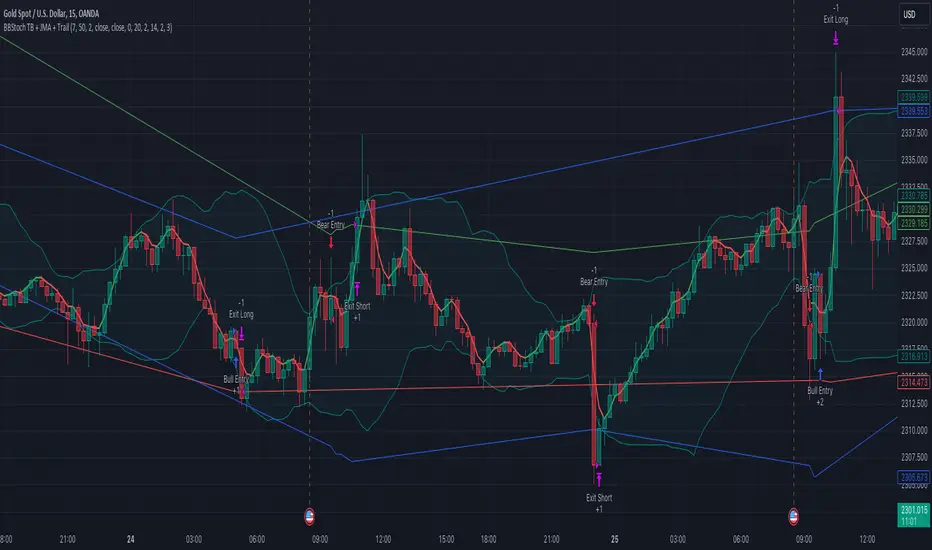
Strategy / Connectable [Azullian]The connectable strategy serves as a foundational component in our indicator system on TradingView, designed for intuitive testing, visualization, and construction of trading strategies. In concert with the connectable signal filter , it forms a cohesive unit that allows for efficient signal processing and strategy implementation. This integration enables the strategy to receive and act on weighted signals from various connectable indicators, making it a versatile tool for both novice and experienced traders.
Let's review the separate parts of this indicator.
█ STRATEGY INPUTS
We've provided an input to connect a signal filter or indicators or chains (→) which is set to 'Close' by default.
An input has several controls:
• Input: Connect indicators or signal filter here, choose indicators with a compatible : Signal connector.
• SM - Signal Mode: Choose a trading direction compatible with the settings in your signal filter
█ POSITION INVESTMENT
Determine the percentage of your trading budget you would like to use in each position based on the strategy's profit or loss.
• LINVB - Loss Investment Base: Choose which base to use to determine the investment percentage when the strategy is in a loss.
○ Equity: Use the equity as the base for percentage calculation.
○ Initial capital: Use the initial capital as the base for percentage calculation.
• LINV% - Loss Investment Percentage: Set a percentage of the chosen investment base as the investment for a new position.
○ For example, when 10% in loss, and a initial capital of $100, and the investment base is set to equity with a percentage of 50%, your investment will be 50% of $90, $45.
• PINVB - Profit Investment Base: Choose which base to use to determine the investment percentage when the strategy is in profit.
○ Equity: Use the equity as the base for percentage calculation.
○ Initial capital: Use the initial capital as the base for percentage calculation.
• PINV% - Profit Investment Percentage: Set a percentage of the chosen investment base as the investment for a new position.
○ For example, when 10% in profit, and an initial capital of $100, and the investment base is set to equity with a percentage of 100%, your investment will be 100% of $110, $110.
• RISK% - Risk Percentage:
○ Determine how much of the calculated position investment is at risk when the stop-loss is hit.
- For example, 1% of $45 represents a maximum loss of $0.45.
○ Risk percentage works together with the stop loss and the max leverage.
• MXLVG - Maximum Leverage:
○ Investigate the trading rules for your trading pair and use the maximum allowed amount of leverage.
○ To determine the number of contracts to be bought or sold, considering the stop loss and the specified risk percentage, the maximum leverage available will constrain the amount of leverage utilized to ensure that the maximum risk threshold is not exceeded. For instance, suppose the stop loss is set at 1%, and the risk percentage is defined as 10%. Initially, the calculated leverage to be used would be 10. However, if there is a maximum leverage cap set at 5, it would constrain the calculated leverage of 10 to adhere to the maximum limit of 5.
█ EXIT STOP LOSS
Determine the Stop Loss price based on your selected configuration.
As the stop loss is an integral part of the ordered contracts calculation used in conjunction with the Risk and Max leverage, you'll always need to provide a stop loss price.
• SLB - Stop Loss Base: Choose a stop loss mode for calculating stop loss prices.
○ Risk: Determines the price using the Risk parameter (RISK%) and maximum leverage (MXLVG). In this case, SLB% will not have any impact.
○ Price Entry + Offset: Calculates the stop loss price based on a offset percentage (SLB%) from the entry price of the position.
• SLB% - Stop Loss Base Percentage: Define an offset percentage that will be applied in the price entry + offset stop loss mode.
• SLT - Stop Loss Trailing:
○ Fixed: The initial stop loss will be kept and no trailing stop loss will be applied.
○ Trail Price: Computes the trailing stop loss price based on an offset percentage (SLT%) from the closing price of the current candle.
- If a better stop loss price is calculated, it will be set as the new stop loss price.
○ Trail Incr: Adapts the trailing stop loss price based on the offset percentage (SLT%).
- Each price change in favor of your position will incrementally adapt the trailing stop loss with SLT%.
• SLT% - Stop Loss Trailing Percentage: This percentage serves as an offset or increment depending on your chosen trailing mode.
█ EXIT TAKE PROFIT
Determine the Take Profit price based on your selected configuration.
• TPB - Take Profit Base: Choose a take profit mode for calculating take profit prices.
○ Reward: Determines the take profit price using the Risk parameter (RISK%) and the calculated Stop Loss price and the set reward percentage (TPB%).
- For example: Risk 1%, Calculated Stop loss price: $90, Entry price: $100, Reward (TPB%): 2%, will result in a take profit price on $120.
○ Price Entry + Offset: Calculates the take profit price based on a offset percentage (TPB%) from the entry price of the position.
- For example: Entry price: $100, Offset (TPB%): 2%, will result in a take profit price on $102.
• TPB% - Take Profit Base Percentage: Define an offset percentage that will be applied in the price entry + offset take profit mode.
• TPT - Take Profit Trailing:
○ Fixed: The initial take profit will be kept and no trailing take profit will be applied.
○ Trail Price: Computes the trailing take profit price based on an offset percentage (TPT%) from the closing price of the current candle.
- If an applicable take profit price is calculated, it will be set as the new take profit price.
○ Trail Incr: Adapts the trailing take profit price based on the offset percentage (TPT%). Each price change against your position will incrementally adapt the trailing take profit with TPT%.
• TPT% - Take Profit Trailing Percentage: This percentage serves as an offset or increment depending on your chosen trailing mode.
█ STRATEGY CONDITIONS
Specify when the strategy is permitted to execute trades.
• DATE: Enable the Date Range filter to restrict entries to a specific date range.
○ START: Set a start date and hour to commence trading.
○ END: Set an end date and hour to conclude trading within the defined range.
■ VISUALS
• LINE: Activate a colored dashed diagonal line to visually connect the entry and exit points of positions.
• SLTP: Enable visualization of stop loss, take profit, and break-even levels.
• PNL: Enable Break-Even and Close Lines along with a colored area in between to visualize profit and loss.
• ☼: Brightness % : Adjust the opacity of the plotted trading visuals.
• P - Profit Color : Choose the color for profit-related elements.
• L - Loss Color: Choose the color for loss-related elements.
• B - Breakeven Color : Select the color for break-even points.
• EL - Long Color: Specify the color for long positions.
• ES - Short Color: Specify the color for short positions.
• TRADE LABELING: For better analysis we've labeled all entries and exits conform with the type of order your strategy has executed, some examples:
○ XL-TP-150: Exit Long - Take Profit - Position 150
○ XS-TP-154: Exit Short - Take Profit - Position 154
○ XL-SL-160: Exit Long - Stop Loss - Position 160
○ XS-SL-164: Exit Short - Stop Loss - Position 164
█ USAGE OF CONNECTABLE INDICATORS
■ Connectable chaining mechanism
Connectable indicators can be connected directly to the signal monitor, signal filter or strategy , or they can be daisy chained to each other while the last indicator in the chain connects to the signal monitor, signal filter or strategy. When using a signal filter you can chain the filter to the strategy input to make your chain complete.
• Direct chaining: Connect an indicator directly to the signal monitor, signal filter or strategy through the provided inputs (→).
• Daisy chaining: Connect indicators using the indicator input (→). The first in a daisy chain should have a flow (⌥) set to 'Indicator only'. Subsequent indicators use 'Both' to pass the previous weight. The final indicator connects to the signal monitor, signal filter, or strategy.
■ Set up the strategy with a signal filter and an RSI indicator
Let's connect the Strategy to a connectable signal filter and a connectable RSI indicator :
1. Load all relevant indicators
• Load RSI / Connectable
• Load Signal filter / Connectable
• Load Strategy / Connectable
2. Signal Filter: Connect the RSI to the Signal Filter
• Open the signal filter settings
• Choose one of the three input dropdowns (1→, 2→, 3→) and choose : RSI / Connectable: Signal Connector
• Toggle the enable box before the connected input to enable the incoming signal
3. Signal Filter: Update the filter signals settings if needed
• The default settings of the filter enable EL (Enter Long), XL (Exit Long), ES (Enter Short) and XS (Exit Short).
4. Signal Filter: Update the weight threshold settings if needed
• All connectable indicators load by default with a score of 6 for each direction (EL, XL, ES, XS)
• By default, weight threshold (TH) is set at 5. This allows each occurrence to score, as the default score in each connectable indicator is 1 point above the threshold. Adjust to your liking.
5. Strategy: Connect the strategy to the signal filter in the strategy settings
• Select the strategy input → and select the Signal filter: Signal connector
6. Strategy: Enable filter compatible directions
• Set the signal mode of the strategy to a compatible direction with the signal filter.
Now that everything is connected, you'll notice green spikes in the signal filter representing long signals, and red spikes indicating short signals. Trades will also appear on the chart, complemented by a performance overview. Your journey is just beginning: delve into different scoring mechanisms, merge diverse connectable indicators, and craft unique chains. Instantly test your results and discover the potential of your configurations. Dive deep and enjoy the process!
█ BENEFITS
• Adaptable Modular Design: Arrange indicators in diverse structures via direct or daisy chaining, allowing tailored configurations to align with your analysis approach.
• Streamlined Backtesting: Simplify the iterative process of testing and adjusting combinations, facilitating a smoother exploration of potential setups.
• Intuitive Interface: Navigate TradingView with added ease. Integrate desired indicators, adjust settings, and establish alerts without delving into complex code.
• Signal Weight Precision: Leverage granular weight allocation among signals, offering a deeper layer of customization in strategy formulation.
• Advanced Signal Filtering: Define entry and exit conditions with more clarity, granting an added layer of strategy precision.
• Clear Visual Feedback: Distinct visual signals and cues enhance the readability of charts, promoting informed decision-making.
• Standardized Defaults: Indicators are equipped with universally recognized preset settings, ensuring consistency in initial setups across different types like momentum or volatility.
• Reliability: Our indicators are meticulously developed to prevent repainting. We strictly adhere to TradingView's coding conventions, ensuring our code is both performant and clean.
█ COMPATIBLE INDICATORS
Each indicator that incorporates our open-source 'azLibConnector' library and adheres to our conventions can be effortlessly integrated and used as detailed above.
For clarity and recognition within the TradingView platform, we append the suffix ' / Connectable' to every compatible indicator.
█ COMMON MISTAKES AND CLARIFICATIONS
• Removing an indicator from a chain: Deleting a linked indicator and confirming the "remove study tree" alert will also remove all underlying indicators in the object tree. Before removing one, disconnect the adjacent indicators and move it to the object stack's bottom.
• Point systems: The azLibConnector provides 500 points for each direction (EL: Enter long, XL: Exit long, ES: Enter short, XS: Exit short) Remember this cap when devising a point structure.
• Flow misconfiguration: In daisy chains the first indicator should always have a flow (⌥) setting of 'indicator only' while other indicator should have a flow (⌥) setting of 'both'.
• Recalculate: While this strategy has undergone extensive testing, enabling recalculation options like 'After order is filled' or 'On every tick' may lead to unexpected behavior.
• Fill orders: The strategy is thoroughly tested, yet enabling fill order options such as 'Using bar magnifier', 'On bar close', or 'Using standard OHLC' might result in unexpected outcomes.
• Layout and abbreviations: To maintain a consistent structure, we use abbreviations for each input. While this may initially seem complex, you'll quickly become familiar with them. Each abbreviation is also explained in the inline tooltips.
• Optimized for crypto trading: While many principles are common across markets, this strategy is specifically optimized and tested for crypto trading.
• Inputs: Connecting a connectable indicator directly to the strategy delivers the raw signal without a weight threshold, meaning every signal will trigger a trade.
█ A NOTE OF GRATITUDE
Through years of exploring TradingView and Pine Script, we've drawn immense inspiration from the community's knowledge and innovation. Thank you for being a constant source of motivation and insight.
█ RISK DISCLAIMER
Azullian's content, tools, scripts, articles, and educational offerings are presented purely for educational and informational uses. Please be aware that past performance should not be considered a predictor of future results.
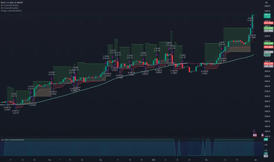
Backtest Strategy Optimizer AdapterBacktest Strategy Optimizer Adapter
With this library, you will be able to run one or multiple backtests with different variables (combinations). For example, you can run 100 backtests of Supertrend at once with an increment factor of 0.1. This way, you can easily fetch the most profitable settings and apply them to your strategy.
To get a better understanding of the code, you can check the code below.
Single backtest results
= backtest.results(date_start, date_end, long_entry, long_exit, take_profit_percentage, stop_loss_percentage, atr_length, initial_capital, order_size, commission)
Add backtest results to a table
backtest.table(initial_capital, profit_and_loss, open_balance, winrate, entries, exits, wins, losses, backtest_table_position, backtest_table_margin, backtest_table_transparency, backtest_table_cell_color, backtest_table_title_cell_color, backtest_table_text_color)
Backtest result without chart labels
= backtest.run(date_start, date_end, long_entry, long_exit, take_profit_percentage, stop_loss_percentage, atr_length, initial_capital, order_size, commission)
Backtest result profit
profit = backtest.profit(date_start, date_end, long_entry, long_exit, take_profit_percentage, stop_loss_percentage, atr_length, initial_capital, order_size, commission)
Backtest result winrate
winrate = backtest.winrate(date_start, date_end, long_entry, long_exit, take_profit_percentage, stop_loss_percentage, atr_length, initial_capital, order_size, commission)
Start Date
You can set the start date either by using a timestamp or a number that refers to the number of bars back.
Stop Loss / Take Profit Issue
Unfortunately, I did not manage to achieve 100% accuracy for the take profit and stop loss. The original TradingView backtest can stop at the correct position within a bar using the strategy.exit stop and limit variables. However, it seems unachievable with a crossunder/crossover function in PineScript unless it is calculated on every tick (which would make the backtesting results invalid). So far, I have not found a workaround, and I would be grateful if someone could solve this issue, if it is even possible. If you have any solutions or fixes, please let me know!
Multiple Backtest Results / Optimizer
You can run multiple backtests in a single strategy or indicator, but there are certain requirements for placing the correct code in the right way. To view examples of running multiple backtests, you can refer to the links provided in the updates I posted below. In the samples I have also explained how you can auto-generate code for your backtest strategy.
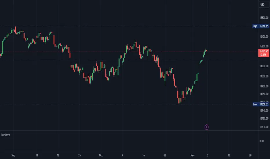
3kilos BTC 15mThe "3kilos BTC 15m" is a comprehensive trading strategy designed to work on a 15-minute timeframe for Bitcoin (BTC) or other cryptocurrencies. This strategy combines multiple indicators, including Triple Exponential Moving Averages (TEMA), Average True Range (ATR), and Heikin-Ashi candlesticks, to generate buy and sell signals. It also incorporates risk management features like take profit and stop loss.
Indicators
Triple Exponential Moving Averages (TEMA): Three TEMA lines are used with different lengths and sources:
Short TEMA (Red) based on highs
Long TEMA 1 (Blue) based on lows
Long TEMA 2 (Green) based on closing prices
Average True Range (ATR): Custom ATR calculation with EMA smoothing is used for volatility measurement.
Supertrend: Calculated using ATR and a multiplier to determine the trend direction.
Simple Moving Average (SMA): Applied to the short TEMA to smooth out its values.
Heikin-Ashi Close: Used for additional trend confirmation.
Entry & Exit Conditions
Long Entry: Triggered when the short TEMA is above both long TEMA lines, the Supertrend is bullish, the short TEMA is above its SMA, and the Heikin-Ashi close is higher than the previous close.
Short Entry: Triggered when the short TEMA is below both long TEMA lines, the Supertrend is bearish, the short TEMA is below its SMA, and the Heikin-Ashi close is lower than the previous close.
Take Profit and Stop Loss: Both are calculated as a percentage of the entry price, and they are set for both long and short positions.
Risk Management
Take Profit: Set at 1% above the entry price for long positions and 1% below for short positions.
Stop Loss: Set at 3% below the entry price for long positions and 3% above for short positions.
Commission and Pyramiding
Commission: A 0.07% commission is accounted for in the strategy.
Pyramiding: The strategy does not allow pyramiding.
Note
This strategy is designed for educational purposes and should not be considered as financial advice. Always do your own research and consider consulting a financial advisor before engaging in trading.
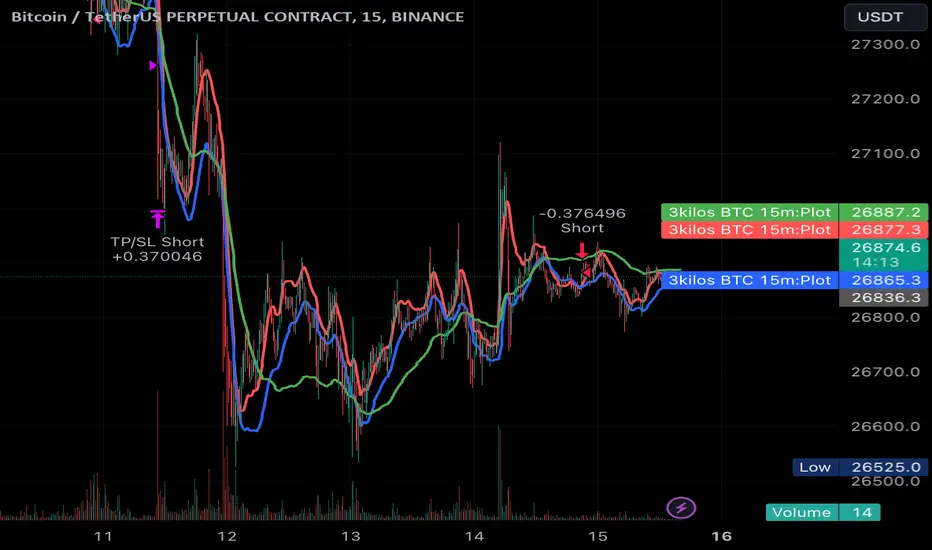
JS-TechTrading: Supertrend-Strategy_Basic versionAre you looking for a reliable and profitable algorithmic trading strategy for TradingView? If so, you might be interested in our Supertrend basic strategy, which is based on three powerful indicators: Supertrend (ATR), RSI and EMA.
Supertrend is a trend-following indicator that helps you identify the direction and strength of the market. It also gives you clear signals for entry and exit points based on price movements.
RSI is a momentum indicator that measures the speed and change of price movements. It helps you filter out false signals and avoid overbought or oversold conditions.
EMA is a moving average indicator that smooths out price fluctuations and shows you the long-term trend of the market. It helps you confirm the validity of your trades and avoid trading against the trend.
Our Supertrend basic strategy combines these three indicators to give you a simple yet effective way to trade any market. Here's how it works:
- For long trades, you enter when the price is above Supertrend and pulls back below it (the low of the candle crosses Supertrend) and then rebounds above it (the high of the next candle goes above the pullback candle). You exit when the price closes below Supertrend or when you reach your target profit or stop loss.
- For short trades, you enter when the price is below Supertrend and pulls back above it (the high of the candle crosses Supertrend) and then drops below it (the low of the next candle goes below the pullback candle). You exit when the price closes above Supertrend or when you reach your target profit or stop loss.
- You can also use RSI and EMA filters to improve your results. For long trades, you only enter if RSI is above 50 and price is above 200 EMA. For short trades, you only enter if RSI is below 50 and price is below 200 EMA.
- You can set your stop loss and target profit as a percentage of your entry price or based on other criteria. You can also adjust the parameters of each indicator according to your preferences and risk tolerance.
Our Supertrend basic strategy is easy to use and has been tested on various markets and time frames. It can help you capture consistent profits while minimizing your losses.
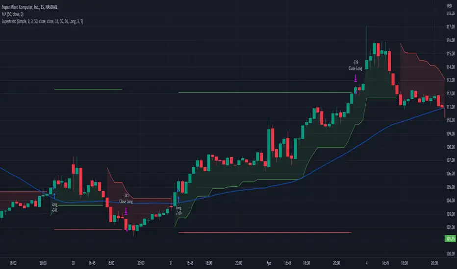
Orion:SagittaSagitta
Sagitta is an indicator the works to assist in the validation of potential long entries and to place stop-loss orders. Sagitta is not a "golden indicator" but more of a confirmation indicator of what prices might be suggesting.
The concept is that while stocks can turn in one bar, it usually takes two bars or more to signal a turn. So, using a measurement of two bars help determine the potential turning of prices.
Behind the scenes, Sagitta is nothing more than a 2 period stochastic which has had its values divided into five specific zones.
Dividing the range of the two bars in five sections, the High is equal to 100 and the Low is equal to 0.
The zones are:
20 = bearish (red) – This is when the close is the lower 20% of the two bars
40 = bearish (orange) – This is when the close is between the lower 20% and 40% of the two bars.
60 = neutral (yellow) – This is when the close is between the middle 40% - 60% of the two bars.
80 = bullish (blue) – This is when the close is between the upper 60% - 80% of the two bars.
100 = bullish (green) – This is when the close is above the upper 80% of the bar.
The general confirmation concept works as such:
When the following bar is of a higher value than the previous bar, there is potential for further upward price movement. Conversely when the following bar is lower than the previous bar, there is potential for further downward movement.
Going from a red bar to orange bar Might be an indication of a positive turn in direction of prices.
Going from a green bar to an orange bar would also be considered a negative directional turn of prices.
When the follow on bar decreases (ie, green to blue, blue to yellow, etc) placing a stop-loss would be prudent.
Maroon lines in the middle of a bar is an indication that prices are currently caught in consolidation.
Silver/Gray bars indicate that a high potential exists for a strong upward turn in prices exists.
Consolidation is calculated by determining if the close of one bar is between the high and low of another bar. This then establishes the range high and low. As long as closes continue with this range, the high and low of the range can expand. When the close is outside of the range, the consolidation is reset.
Signals in areas of consolidation (maroon center bar) should be looked upon as if the prices are going to challenge the high of the consolidation range and not necessarily break through.
The entry technique used is:
The greater of the following two calculations:
High of signal bar * 1.002 or High of signal bar + .03
The stop-loss technique used is:
The lesser of the following two calculations:
Low of signal bar * .998 or Low of signal bar - .03
IF an entry signal is generated and the price doesn’t reach the entry calculation. It is considered a failed entry and is not considered a negative or that you missed out on something. This has saved you from losing money since the prices are not ready to commit to the direction.
When placing a stop-loss, it is never suggested that you lower the value of a stop-loss. Always move your stop-losses higher in order to lock in profit in case of a negative turn.
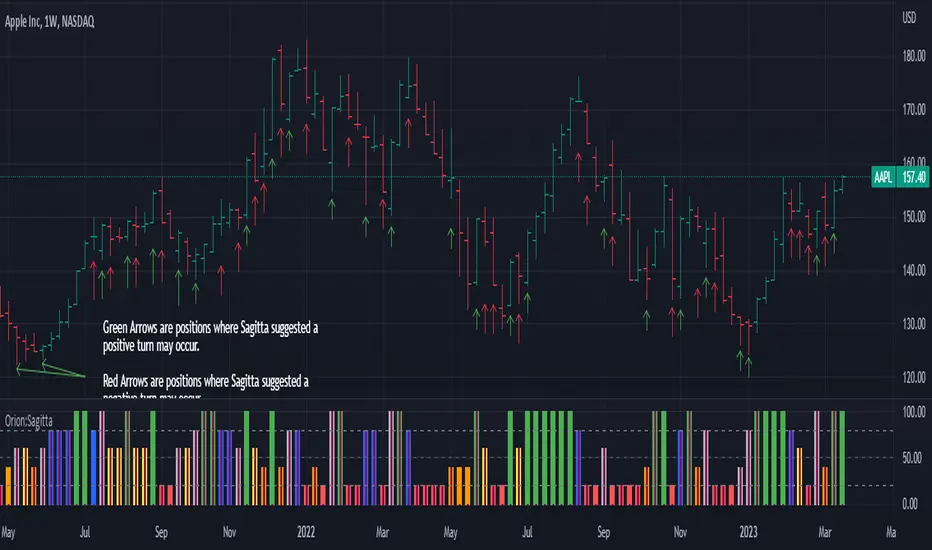
Investments/swing trading strategy for different assetsStop worrying about catching the lowest price, it's almost impossible!: with this trend-following strategy and protection from bearish phases, you will know how to enter the market properly to obtain benefits in the long term.
Backtesting context: 1899-11-01 to 2023-02-16 of SPX by Tvc. Commissions: 0.05% for each entry, 0.05% for each exit. Risk per trade: 2.5% of the total account
For this strategy, 5 indicators are used:
One Ema of 200 periods
Atr Stop loss indicator from Gatherio
Squeeze momentum indicator from LazyBear
Moving average convergence/divergence or Macd
Relative strength index or Rsi
Trade conditions:
There are three type of entries, one of them depends if we want to trade against a bearish trend or not.
---If we keep Against trend option deactivated, the rules for two type of entries are:---
First type of entry:
With the next rules, we will be able to entry in a pull back situation:
Squeeze momentum is under 0 line (red)
Close is above 200 Ema and close is higher than the past close
Histogram from macd is under 0 line and is higher than the past one
Once these rules are met, we enter into a buy position. Stop loss will be determined by atr stop loss (white point) and break even(blue point) by a risk/reward ratio of 1:1.
For closing this position: Squeeze momentum crosses over 0 and, until squeeze momentum crosses under 0, we close the position. Otherwise, we would have closed the position due to break even or stop loss.
Second type of entry:
With the next rules, we will not lose a possible bullish movement:
Close is above 200 Ema
Squeeze momentum crosses under 0 line
Once these rules are met, we enter into a buy position. Stop loss will be determined by atr stop loss (white point) and break even(blue point) by a risk/reward ratio of 1:1.
Like in the past type of entry, for closing this position: Squeeze momentum crosses over 0 and, until squeeze momentum crosses under 0, we close the position. Otherwise, we would have closed the position due to break even or stop loss.
---If we keep Against trend option activated, the rules are the same as the ones above, but with one more type of entry. This is more useful in weekly timeframes, but could also be used in daily time frame:---
Third type of entry:
Close is under 200 Ema
Squeeze momentum crosses under 0 line
Once these rules are met, we enter into a buy position. Stop loss will be determined by atr stop loss (white point) and break even(blue point) by a risk/reward ratio of 1:1.
Like in the past type of entries, for closing this position: Squeeze momentum crosses over 0 and, until squeeze momentum crosses under 0, we close the position. Otherwise, we would have closed the position due to break even or stop loss.
Risk management
For calculating the amount of the position you will use just a small percent of your initial capital for the strategy and you will use the atr stop loss for this.
Example: You have 1000 usd and you just want to risk 2,5% of your account, there is a buy signal at price of 4,000 usd. The stop loss price from atr stop loss is 3,900. You calculate the distance in percent between 4,000 and 3,900. In this case, that distance would be of 2.50%. Then, you calculate your position by this way: (initial or current capital * risk per trade of your account) / (stop loss distance).
Using these values on the formula: (1000*2,5%)/(2,5%) = 1000usd. It means, you have to use 1000 usd for risking 2.5% of your account.
We will use this risk management for applying compound interest.
In settings, with position amount calculator, you can enter the amount in usd of your account and the amount in percentage for risking per trade of the account. You will see this value in green color in the upper left corner that shows the amount in usd to use for risking the specific percentage of your account.
Script functions
Inside of settings, you will find some utilities for display atr stop loss, break evens, positions, signals, indicators, etc.
You will find the settings for risk management at the end of the script if you want to change something. But rebember, do not change values from indicators, the idea is to not over optimize the strategy.
If you want to change the initial capital for backtest the strategy, go to properties, and also enter the commisions of your exchange and slippage for more realistic results.
If you activate break even using rsi, when rsi crosses under overbought zone break even will be activated. This can work in some assets.
---Important: In risk managment you can find an option called "Use leverage ?", activate this if you want to backtest using leverage, which means that in case of not having enough money for risking the % determined by you of your account using your initial capital, you will use leverage for using the enough amount for risking that % of your acount in a buy position. Otherwise, the amount will be limited by your initial/current capital---
Some things to consider
USE UNDER YOUR OWN RISK. PAST RESULTS DO NOT REPRESENT THE FUTURE.
DEPENDING OF % ACCOUNT RISK PER TRADE, YOU COULD REQUIRE LEVERAGE FOR OPEN SOME POSITIONS, SO PLEASE, BE CAREFULL AND USE CORRECTLY THE RISK MANAGEMENT
Do not forget to change commissions and other parameters related with back testing results!
Some assets and timeframes where the strategy has also worked:
BTCUSD : 4H, 1D, W
SPX (US500) : 4H, 1D, W
GOLD : 1D, W
SILVER : 1D, W
ETHUSD : 4H, 1D
DXY : 1D
AAPL : 4H, 1D, W
AMZN : 4H, 1D, W
META : 4H, 1D, W
(and others stocks)
BANKNIFTY : 4H, 1D, W
DAX : 1D, W
RUT : 1D, W
HSI : 1D, W
NI225 : 1D, W
USDCOP : 1D, W